Cosine Similarity and Intrinsic Dimension

The cosine measure is the prevailing similarity function for the document vector model of IR. We discuss a its connection to the intrinsic dimension.

Mostly only two reasons are given for choosing the cosine measure: Comuptational efficiency and favorable modelling properties. But there is annother important reason, namely reducing the intrinsic dimension of the vector space.

Introduction

The cosine measure is the prevailing similarity function for the document vector model of information retrieval, see Salton1975 (1). Very often only two reasons are given for choosing the cosine measure as a similarity function:

• Firstly, because the cosine can efficently be calculated as the dot product of two document vectors, and
• secondly, in the text retrieval context a similarity measure based on the angle seems more suitable, since the document length should not influence the similarity of two documents, see Salton 1988, p. 517 (2) and Manning et.al. 2008 (3).

Not so often following motivation for using a semimetric (the triangle inequality doesn't hold, see section Cosine Similarity for a discussion) is given.

• Lets imagine a centaur. Now it seems reasonable that a man as well as a horse is closely related to a centaur. But a horse and a man are much less related so that the triangle inequality of a full metric space is violated. You can easily come up with more examples. E.g. consider nurse - doctor - woman. The semantic distance between doctor - woman seems to be much larger than the sum of distances doctor - nurse plus nurse - woman. This phenomenon seems to be a natural property of languange.

• But there still is another important motivation for the use of the cosine similarity, which consequently may fosters the application of cluster algotrithms. The latter is due the fact, that cluster algorithms try to maximize inter (between) cluster distances and at the same time minimize intra (within) cluster distances. The property of the semimetric induced by the cosine similarity helps this optimization procedure by decreasing the distance between similar and increasing the distance of dissimilar objects, see section Intrinsic Dimension for a discussion.

Cosine Similarity

The similarity between two document vectors $d_i$ and $d_j$ is calculated as the cosine of the enclosed angle $\theta = \angle(d_i, d_j)$:

$$ sim(d_i, d_j) = cos(\theta) = \frac{d_i^T d_i}{\|d_i\|\cdot \|d_j\|}. $$

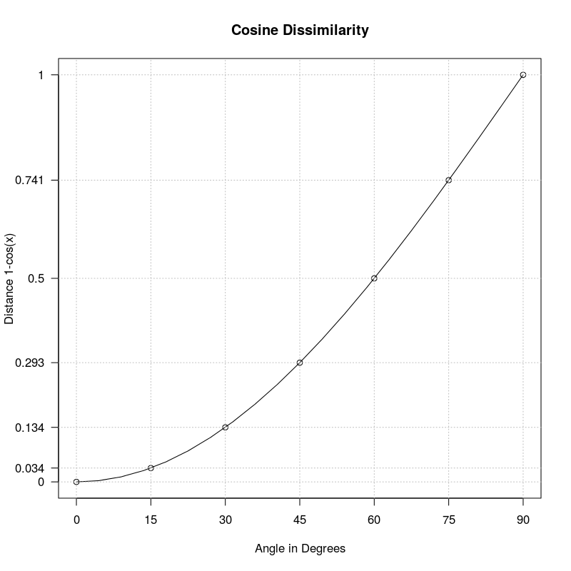
The dissimilarity funtion $1-cos(\theta)$ induced by cosine similariy is not a metric but semi-metric. That is the triangle inequality doesn't hold. This is clear when we look at the functional form of $1-cos(\theta)$:

To (re)produce the above image you can use the following R script:

 # change to working directory
 setwd("~/Pictures")
 # domain values for x 
 x = seq(0,pi/2,length.out=21)
 # x-axes and y-axes labels to print
 x_label_val = seq(0,pi/2,length.out=7)
 x_label_print = 2*x_label_val/pi*90
 y_label_val = 1.0-cos(x_label_val)
 # plot plot graph
 png("cosine.png", width = 800, height = 800, res=100)
 plot(x,1-cos(x), t="l", main="Cosine Dissimilarity", xlab="Angle in Degrees",
    ylab="Distance 1-cos(x)",xaxt="n", yaxt="n");
 lines(x_label_val,1-cos(x_label_val), t="p");
 # print x-axis and y-axis
 axis(1,x_label_val,labels=x_label_print)
 axis(2,y_label_val,labels=round(y_label_val,3),las=1)
 # print grid lines
 abline(h=y_label_val, col="grey", lty=3)
 abline(v=x_label_val, col="grey", lty=3)
 dev.off()

Lets look at three vectors a, b and c where $$\angle(a, b)=\angle(b, c)=15^\circ,\quad\angle(a, c)=30^\circ.$$

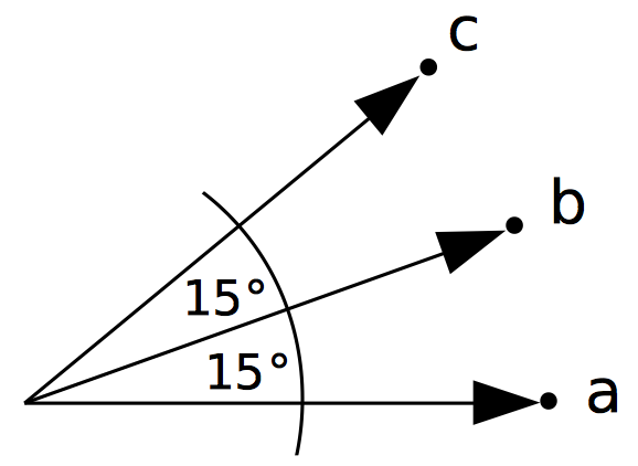
From the plot of angles versus cosine distance above wee see that $$d(a,b)=d(b,c)\approx 0.034,\quad d(a,c)\approx 0.134.$$ So $$d(a,b)+d(b,c)\lt d(a,c)$$ which obviously violates the triangle inequality which postualtes $$ d(a,b)+d(b,c) \geq d(a,c).$$

Intrinsic Dimension

When we consider a document collection as a set of points (vectors) in a vector space we have to consider different definitions of dimension.

• Firstly there is the algebraic dimension, which equals the number of terms in the vocabulary and is very high dimensional (often millions).
• On the other hand the data set may lie in a very small hyperspace, e.g. a plane (very unlikely). When trying to build an index this latter intrinsic dimension plays a key role, since it helps us with issues stemming from the curse of dimensionality.

One way to define an intrinsic dimension is the following:

\begin{equation} \rho = \frac{\mu^2}{2\sigma^2}, \end{equation}

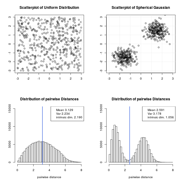
where $\mu$ is the average distance between two document vectors and $\sigma^2$ the variance of the pairwise distances, for details see Skobal et.al. 2004 (4). In other words, if all pairs of document vectors are almost equally distant (the data set is uniformly distributed) $\sigma$ becomes small and therefore the dimension $\rho$ becomes large. On the other hand if the distance between nearby points is small (intra cluster distance) and the distance between further distant vectors is big (inter cluster distance) the mean gets faster smaller than the variance which in turn decreases the dimension $\rho$. Skobal et.al. (4) write:

On the other side, the convex modifications [...] even more tighten the object clusters, making the cluster structure of the dataset more evident. Simply, the convex modifications increase the distance histogram variance, thereby decreasing the intrinsic dimensionality.

Lets look at an synthetic example in the 2-dimensional plane:

Here is the R-project code to drqa the above plot:

library("MASS")
plot_rho = function(s1, s2, t1, t2) {
    d1 = dist(s1)
    d2 = dist(s2)
    rho1 = mean(d1)^2 / (2 * var(d1))
    rho2 = mean(d2)^2 / (2 * var(d2))
    par(mfrow=c(2,2)) # combine plots in 2 x 2 layout
    limits = c(-3,3) # limits for scatter plot
    plot(s1, xlab="", ylab="", main=sprintf("Scatterplot of %s", t1), xlim=limits, ylim=limits); grid()
    plot(s2, xlab="", ylab="", main=sprintf("Scatterplot of %s", t2), xlim=limits, ylim=limits); grid()
    hist(d1[d1 < 8], breaks=seq(0,8,by=0.2), ylim=c(0,15000), main="Distribution of pairwise Distances", xlab="pairwise distance", ylab="")
    abline(v = mean(d1), col = "royalblue", lwd = 2)
    legend("topright", c(sprintf("Mean %.3f", mean(d1)),sprintf("Var %.3f", var(d1)),sprintf("intrinsic dim. %.3f", rho1)))
    hist(d2[d2 < 8], breaks=seq(0,8,by=0.2), ylim=c(0,15000), main="Distribution of pairwise Distances", xlab="pairwise distance", ylab="")
    abline(v = mean(d2), col = "royalblue", lwd = 2)
    legend("topright", c(sprintf("Mean %.3f", mean(d2)),sprintf("Var %.3f", var(d2)),sprintf("intrinsic dim. %.3f", rho2)))
 }
 #
 # spherical normal distribution
 #
 Sigma = matrix(c(0.25,0,0,0.25),2,2) 

 s_sphere1 = mvrnorm(n = 250, c(-1.5,-1.5), Sigma) # sample multivariate normal with correlation matrix Sigma
 s_sphere2 = mvrnorm(n = 250, c(1.5,1.5), Sigma) # sample multivariate normal with correlation matrix Sigma
 s_sphere = rbind(s_sphere1, s_sphere2)
 #
 # Uniform random numbers
 #
 s_uni = matrix(runif(1000, -3,3), nrow=500)
 setwd("~/Pictures")
 png("intrinsic_dim.png", width = 800, height = 800, res=100)
 plot_rho(s_uni, s_sphere, "Uniform Distribution", "Spherical Gaussian")
 dev.off()

Summary

In structured high dimensional vector spaces the cosine similarity helps to reduce the intrinsic dimension and therefore helps to avoid or reduce problems connected to the curse of dimensionality. For example clustering algorithms in the vector space model of information retrieval may benefit from this property.

Bibliography

[1] Gerard Salton, A. Wong, C. S. Yang. A vector space model for automatic indexing. Commun. ACM 18(11): 613-620 (1975).
[2] Gerard Salton and Christopher Buckley. Term-weighting approaches in automatic text retrieval. Elsevier, Information Processing and Management, Volume 24, Issue 5 (1988).
[3] Manning, Christopher D. and Raghavan, Prabhakar and Schütze, Hinrich. Introduction to Information Retrieval". Cambridge University Press 2008.
[4] Tomáš Skopal, Pavel Moravec, Jaroslav Pokorný, Václav Snášel Metric Indexing for the Vector Model in Text Retrieval. String Processing and Information Retrieval: 11th International Conference, SPIRE 2004, Padova, Italy, October 5-8, 2004. Proceedings.