The binomial options pricing model provides a numerical method for the valuation of options. Here I will give a short introduction to option pricing using the binomial tree model proposed by Cox, Ross and Rubinstein in 1979 (1).
Contents
The basic idea of an option reaches back at least to the hellenistic philosophers. Aristoteles writes in his book one Politics, Part XI (thanks to Peter Forsyth (2) for this nice example, apart from Aristoteles I mean):
There is the anecdote of Thales the Milesian and his financial device, which involves a principle of universal application, but is attributed to him on account of his reputation for wisdom. He was reproached for his poverty, which was supposed to show that philosophy was of no use. According to the story, he knew by his skill in the stars while it was yet winter that there would be a great harvest of olives in the coming year; so, having a little money, he gave deposits for the use of all the olive-presses in Chios and Miletus, which he hired at a low price because no one bid against him. When the harvest-time came, and many were wanted all at once and of a sudden, he let them out at any rate which he pleased, and made a quantity of money. Thus he showed the world that philosophers can easily be rich if they like, but that their ambition is of another sort.
Applying this trading strategy the most Thales could lose was the deposits on the olive mills. On the other hand when the demand was high (after a great harvest and since olives could not be stored for long) he would make a big profit by subletting the presses. In more modern terms he constructed a call option on the future price of olives. But also note, that Thales used his extraordinary skills to predict the height of the next harvest and thus make a profit by applying the above sketched strategy. Without his exclusive inside, even the most intricate trading strategy will not guarantee a profit above the Risk-free Interest Rate: There ain't no such thing as a free lunch or in financial terms, arbitrage would eliminate any systematic profits above the risk-free rate.
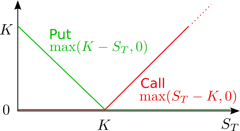
An European put option gives the holder the right to sell the underlying stock or commodity at a future point of time $T$ for a fixed price $K$. Analogous an European call option gives the holder the right to buy the underlying stock or commodity at a future point of time $T$ for a fixed price $K$. Both options are charaterised by
As it is clear from the above definition a put will pay off, when the price of the underlying assets drops below the strike price at time $T$. So the put can be seen as an insurance against falling prices. In contrast a call pays off when the price rises above the strike price at maturity, so we can use a call to speculate on rising prices. Also note that if we are holding both a call and a put with the same characteristics, there payoffs cancle each other out.
We introduced put and call options but we don't know how to calculate a fair price for such derivative contracts. Using the binomial tree approach we will learn some important concepts of mathematical finance notably the principle of no arbitrage.
The following example is motivated by John Hull's widely used text book Options, futures, and other derivatives (3), but can be found in any introductionary text on option pricing as in Peter Forsyth's An introduction to Computational Finance without Agonizing Pain (4).
Let us assume we want to value an European put option on an underlying stock $S$ with strike price $K:=€19$. To make things simple we assume that we are in a simple one time-step, two state world. The precise example is shown below.
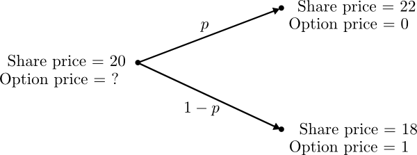
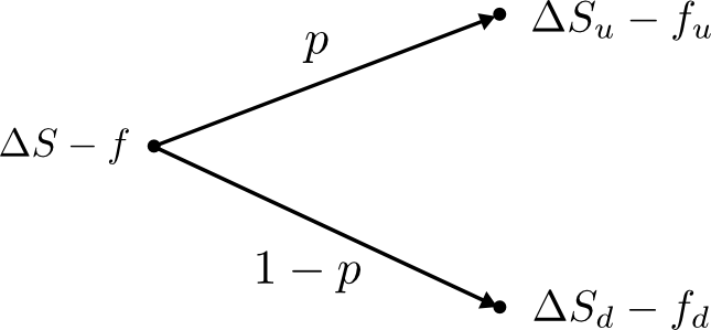
Ignore $p$ for time being - we'll later come back to it. Now our agenda is to construct a portfolio consisting of a position in $\Delta$ shares and a short position in the put option. A short position simply means selling an asset. If we can choose $\Delta$ so that the portfolio becomes risk-free, we then could calculate the option price $f$ using an arbitrage-free argument. The situation is depicted below and we will describe the two step in more detail in the following.
What do we mean by (financial) risk? Let's say we own some asset (a stock, a bond, a commodity, etc.) which has a price $S_0$ today. Since the future price $S_1$ is uncertain we are bearing a risk. If you don't want to bear any risk you would buy a risk-free asset like a high rated government bond (naturally, a goverment bond is in reality not fully risk-free, but it is the best we can do). Looking at it from annother angle, we say
a financial portfolio is per definition risk-free, if its values for all possible future states are equal.
Here this means that our portfolio is equal in both future states:
\begin{equation} \Delta S_u - f_u = \Delta S_d - f_d \Rightarrow \Delta = \frac{f_u - f_d}{S_u - S_d}.\label{eq:delta} \end{equation}
In our example we quickly verify using \eqref{eq:delta} that
\begin{equation}\label{eq:delta2} \Delta=(0-1)/(22-18)=-0.25. \end{equation}
We now set up a portfolio P consisting of a short position in $\Delta$ shares of stock and a short position in the option. Since we want it to be risk-free and we assume no arbitrage possibilities it must earn the risk-free rate of interest (see discussion Arbitrage and Risk-Free Rate). That is, after time period $T$, $e^{rT}P_0=P_1$:
\begin{align} e^{rT} (\Delta S - f) &= \Delta S_u - f_u\nonumber\newline \Rightarrow f &= \Delta S - e^{-rT}(\Delta S_u - f_u)\label{eq:risk-free-cond} \end{align}
Putting \eqref{eq:delta2} into \eqref{eq:risk-free-cond}, setting the risk-free rate $r:=3\%$ and the length of one time-step to three month, we get:
\begin{align} f &= -0.25\cdot €20 - e^{-0.03\cdot 0.25}(-0.25\cdot €22)\nonumber\newline &= -€5 - 0.992528\cdot (-€5.5)\nonumber\newline &= €0.4589. \label{eq:calc1} \end{align}
So our price for our Eurpean put option with maturity 3 month and a strike price of $K=€19$ and $S=€20$ is approx. 46 cent.
Let us sell $\Delta$ shares of the stock and sell one option. We invest the receits in a riskless money account $B_0 = \Delta S_0 + f$:
$$ B_0 = \Delta S_0 + f = 0.25\cdot €20 + €0.4589 = €5.4589. $$
You might wonder, how we could sell a stock we don't own. Among financial players it is common that one firm lends annother firm some shares for a certain time period without any costs. The lender only request, depending on the price movements of the asset, a certain amount in order not to be exposed to counter party risk (the risk the partner will not be able to return the asset shares). This amount is called a margin. We could pay the margin using our bank account. For further details please consult John Hull (3), or other text book.
In the absence of arbitrage opportunities, a risk-free portfolio must earn the risk-free rate of interest. Otherwise we could bag a risk-free profit. This seems intuitively clear, but let us make this explicit:
In both cases we could make a risk-free profit, which contradicts our assumption that markets lack arbitrage possibilities.
We will continue our investigation in the next post where we will among others learn what risk-neutral pricing is all about.
Arbitage is the possibility of a risk-free profit (after transaction costs). More precisely, if the probability for a loss is zero and the probability for a profit is strictly greater than zero, we call the trading strategy an arbitrage.
The concept is best understood by the following joke (5):
A finance professor and a normal person go on a walk, and the normal person sees a € 100 bill lying on the street. When the normal person wants to pick it up, the finance professor says: “Don’t try to do that. It is absolutely impossible that there is a € 100 bill lying on the street. Indeed, if it were lying on the street, somebody else would already have picked it up.”
An arbitage-free market is a market without arbitrage opportunities. We alway assume the absence of arbitrage opportunities. For certain transparent markets this seems a reasonable assumptions, since any arbitrage opportunitie will be quickly exploited so that they vanish. Indeed, big financial institution usually have own units to find and exploit arbitrage possibilities. Anyone remember Nick Leeson who brought down Barings Bank? He was an Arbitageur.
The risk-free interest rate is the interest that market participants are ready to pay for a risk-less loan. Sometimes the rates of government bonds are used as proxies for the risk-free rate but traders usually use the LIBOR as a proxy.


Consider an amount A beeing invested for $t$ years at an interest rate of R per annum. The terminal value of the investment clearly is
$$A(1+R)^t$$
Now imagine we are compunding in ever smaller time steps, like monthly, daily and so on. Then the accrued value of the investment after $t$ years and $n$ time steps per year is
$$A\left(1+\frac{R}{n}\right)^{tn}.$$
For example with a monthly compounded interest rate for a €100 investment and 3% yearly interest rate the investment grows after the first year to
$$€100\cdot(1+0.0025)^{12}\approx €103.0416,$$
where $0,0025 = 3\% / 12$. Taking the limit in the compounding frequency $n$ is called continous compounding. The limit of the amount after $t$ years with continous interest rate $R$ can be calculated as
\begin{align*} \lim_{n\rightarrow\infty}A\left(1+\frac{R}{n}\right)^{tn} &= A\exp\left(\lim_{n\rightarrow\infty} tn \ln\left(1+\frac{R}{n}\right)\right)\newline &= A\exp\left(Rt\lim_{n\rightarrow\infty} \frac{\ln\left(1+\frac{R}{n}\right)}{\frac{R}{n}}\right)\newline &= A\exp\left(Rt\frac{d}{dx}\ln 1\right)\newline &= A\exp (Rt)= Ae^{Rt}, \end{align*}
where we used $\exp(\ln(x))=x$, $\,\ln'(x)=1/x\Rightarrow \ln'(1)=1$ and the continuity of the limit. For example an investment of €1 today and a yearly continous rate of 3% would be worth $€1\cdot e^{(1\cdot 0.03)}\approx €1.030454$ in one year and $€1\cdot e^{(10\cdot 0.03)}\approx €1.349859$ in 10 years.
Remember the exponential function? Here is a graph of $\exp(x) = e^x$:
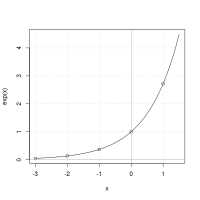
R code to (re)produce the plot.
x  = seq(-3, 1.5, 0.1)
x2 = seq(-3, 1.5, 1)
plot(x,exp(x),type="l")
lines(x2,exp(x2), t="p")
abline(h = 0, v = 0, col = "gray60"); grid()
Bibliography
[1] Cox, Ross and Rubinsteinr. Option Pricing: A Simplified Approach, Journal of Financial Economics 7: 229-263, 1979,
[2] Peter Forsyth 2003: An introduction to Computational Finance.
[3] John C. Hull: "Options, Futures and Other Derivatives", 6th edition, Prentice Hall 2006
[4] Peter Forsyth 2008: An introduction to Computational Finance without Agonizing Pain.
[5] Freddy Delbaen and Walter Schachermayer: What is a Free Lunch? Notes on the AMS, Volume 51, Number 5.