Option Pricing Using Binomial Trees 2

In this part we will continue our one time-step two states binomial tree model for pricing an option (previous post) which will leed us to the principle of risk-neutral valuation.

Contents

1. Summary of Part 1
2. Risk-Neutral Valuation

Summary of Part 1

Let us first summarize the main results from part 1

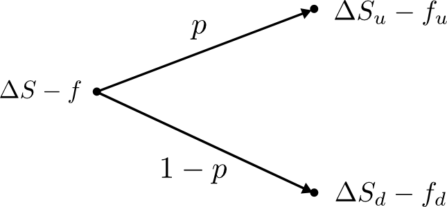
1. Construct a risk-free portfolio consisting of a long position in $\Delta$ shares and a short position in the put option:

   \begin{align} \Delta S_u - f_u &= \Delta S_d - f_d \nonumber\newline \Rightarrow \Delta &= \frac{f_u - f_d}{S_u - S_d}.\label{eq:delta} \end{align}

2. Assuming an arbitrage-free market, a risk-free portfolio must earn the risk-free rate and using \eqref{eq:risk-free-cond}:

   \begin{align} e^{rT} (\Delta S - f) &= \Delta S_u - f_u\nonumber\newline \Rightarrow f &= \Delta S - e^{-rT}(\Delta S_u - f_u)\label{eq:risk-free-cond} \end{align}

Risk-Neutral Valuation

Let us introduce

• $u:=\frac{S_u}{S}$ where $u$ stands for up and
• $d:=\frac{S_d}{S}$ where $d$ stands for down.

Then we can rewrite \eqref{eq:risk-free-cond} as follows

\begin{equation}\label{eq:rewrite} f = \Delta S-e^{-rT}(\Delta Su-f_u). \end{equation}

Substituting $\Delta$ from \eqref{eq:delta} in \eqref{eq:rewrite} gives:

\begin{align} f &= \frac{f_u -f_d}{u-d} - e^{-rT}\left(\frac{f_u -f_d}{u-d}u-f_u\right)\nonumber\newline &= \frac{f_u -f_d}{u-d} - e^{-rT}\left(\frac{f_uu -f_du - f_uu + f_ud}{u-d}\right)\nonumber\newline &= e^{-rT}\left(\frac{e^{rT}f_u -e^{rT}f_d + f_du - f_ud }{u-d}\right)\nonumber\newline &= e^{-rT}\left(\frac{e^{rT} -d}{u-d}f_u + \frac{-e^{rT}+u}{u-d}f_d\right)\nonumber \end{align}

and finally we get

\begin{equation}\label{eq:expected_payoff} f = e^{-rT}(pf_u + (1-p)f_d) \end{equation}

where

\begin{equation}\label{eq:prop} p := \frac{e^{rT} -d}{u-d} \end{equation}

Let`s calculate the put price again, this time using our new equation \eqref{eq:expected_payoff}. With $K=19$, $S=20$, $S_u=22$ and $S_d=18$ we have

\begin{align*} u &= 22/20 = 1.1\newline d &= 18/20 = 0.9\newline e^{-rT} &=e^{0.03\cdot 0.25}=0.992528\newline e^{rT} &=e^{-0.03\cdot 0.25}=1.007528\newline p &= (1.007528-0.9)/0.2 = 0.537640\newline \Delta &= (f_u-f_d)/(S_u-S_d) = -0.25, \end{align*}

so that we finally get for the option price

\begin{equation} f = 0.992528(0.53754\cdot 0 + (1-0.53754)\cdot 1) = 0.4590.\nonumber \end{equation}

It doesn't surprise us, that this is the value we calculated before in the previous part using equation \eqref{eq:risk-free-cond} (apart from rounding errors).

It seems intuitive to interprete the parameter $p$ as the propability of the stock to move from €20 to €22. Indeed with this interpretation equation \eqref{eq:expected_payoff} becomes the discounted expected value of the future payoffs. Let's see if we can make a similar statement for the expected value of the stock:

\begin{align} E(S_T) &= pS_0u + (1-p)S_0d\nonumber\newline &= pS_0(u-d) +S_0d\nonumber \end{align}

leading to

\begin{equation}\label{eq:expectation_asset} E(S_T)= S_0e^{rT} \end{equation}

or respectively

\begin{equation}\label{eq:expectation_asset2} S_0 = e^{-rT}E(S_T). \end{equation}

So when we follow our assumptions for pricing the option, all assets earn the risk-free rate of interest. In other words an investor expects the same return on any asset regardless of the involved risk. Such an investor is called risk-neutral. It contrast to a real-life investor, who expects more return on a risky investment - he is risk-averse (this contrasts again to a gambler who generally is risk-seeking). Lets summarize our results with the words of John C. Hull:

In a risk-neutral world all individuals are indifferent to risk. They require no compensation for risk, and the expected return on all securities is the risk-free interest rate. Equation \eqref{eq:expectation_asset} shows that we are assuming a risk-neutral world when we set the propability of an up movement to $p$. Equation \eqref{eq:expected_payoff} shows that the value of the option is its expected payoff in a risk-neutral world discounted at the risk-free rate. (1, p. 205)

We will continue our investigation in the next post where we will determine the future up and down movement of the stock or equivalently the probability $p$ as can be seen from equation \eqref{eq:prop}.

Bibliography

[1] John C. Hull: "Options, Futures and Other Derivatives", 4th edition, Prentice Hall 2000