Option Pricing Using Binomial Trees 3

In the previous article we showed how to price an option using the risk-neutral valuation principle. Following this principle the arbitrage-free option price is the expected payoff discounted by the risk-free interest rate. What we were missing until now is how to calculate the risk-neutral propability $p$.

Contents

1. Matching the Stock Price Volatility
2. Examples
   1. European Call
   2. European Put

Matching the Stock Price Volatility

First we want our tree to match the given expected return of the stock which has to be the risk-free interest rate following the above risk-neutral valuation approach.

\begin{equation} Se^{r\Delta t} = pSu+(1-p)Sd\quad\Rightarrow\quad p=\frac{e^{r\Delta t}-d}{u-d}. \label{solution1} \end{equation}

Secondly we want to match the given yearly volatility $\sigma$ of the return of the stock price. Now let $X$ be the stochastic return given by

\begin{align*} X :=& \left\{ \begin{array}{ll} u-1 & \text{with probability } p\newline d-1 & \text{with probability } 1-p\newline \end {array}\right.\newline \quad\Rightarrow\quad X+1 =& \left\{ \begin{array}{ll} u & \text{with probability } p\newline d & \text{with probability } 1-p\newline \end{array}\right. \end{align*}

then using $Var(X+1) = Var(X)$, $Var(X)=E(X^2)-E(X)^2$ and $\sigma^2\Delta t=Var(X)$:

\begin{align} \sigma^2\Delta t &= pu^2+(1-p)d^2 -\left(pu+(1-p)d\right)^2\nonumber\newline &= pu^2+ud+(1-p)d^2-ud-e^{2r\Delta t}\nonumber\newline &= (pu+(1-p)d)(u+d) - ud -e^{2r\Delta t}\nonumber\newline &= e^{r\Delta t}(u+d) - ud -e^{2r\Delta t}.\label{lab1} \end{align}

Since for small positiv $x$ we have $e^x\approx 1+x$ (remember $e^x=1+x+\frac{x^2}{2!}+\cdots$) one solution for $u$, $d$ is given by

\begin{align} u &= e^{\sigma\sqrt{\Delta t}}\nonumber\newline d &= e^{-\sigma\sqrt{\Delta t}}\label{solution2} \end{align}

To see that the above values for $u$ and $d$ are really a solution, just plug them into the right side of equation $\eqref{lab1}$:

\begin{align}\label{lab2} \eqref{lab1} & = e^{r\Delta t}(e^{\sigma\sqrt{\Delta t}}+e^{-\sigma\sqrt{\Delta t}}) - e^{\sigma\sqrt{\Delta t}}e^{-\sigma\sqrt{\Delta t}} - e^{2r\Delta t}\nonumber\newline & \approx (1+r\Delta t)((1+\sigma\sqrt{\Delta t}) + (1-\sigma\sqrt{\Delta t}))\nonumber\newline & \qquad - (1+\sigma\sqrt{\Delta t})(1-\sigma\sqrt{\Delta t}) - (1+2r\Delta t) \nonumber\newline & = 2 + 2r\Delta t - 1 + \sigma^2\Delta t - 1 - 2r\Delta t = \sigma^2\Delta t. \end{align}

Given the risk-free interest rate $r$ and the volatility $\sigma$ of the underlying asset we can calibrate the binomial tree using $\eqref{solution1}$ and $\eqref{solution2}$:

\begin{align} u &= e^{\sigma\sqrt{\Delta t}}\nonumber\newline d &= e^{-\sigma\sqrt{\Delta t}}\label{calibration}\newline p &= \frac{e^{r\Delta t}-d}{u-d}.\nonumber \end{align}

Examples

European Call

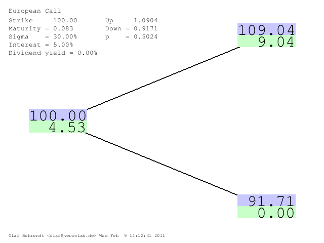
Now lets assume the following values

$$ S = 1,\ K=1,\ T=1/12=0.0833,\ r = 5\%,\ \sigma=30\% $$

1. First we have to calibrate our tree model using $\eqref{calibration}$ and the above values: \begin{equation*} \begin{split} u &= e^{\sigma\sqrt{\Delta t}}=e^{0.3\sqrt{0.0833}}=1.0904\newline d &= e^{-\sigma\sqrt{\Delta t}}=e^{-0.3\sqrt{0.0833}}=0.9171\newline p &=\frac{e^{r\Delta t}-d}{u-d}=\frac{1.0042-0.9171}{1.0904-0.9171}=0.5026 \end{split} \end{equation*}
2. Next we calculate the payoff values for each state: \begin{align*} V_1^{up} &= \max(Su-K,0)=\max(1.0904-1.0,0)=0.0904\newline V_1^{down} &= \max(Sd-K,0)=\max(0.9171-1.0,0)=0.0 \end{align*}
3. Finally the option price is given by the discounted expected value of the future payoffs: \begin{align*} V_0 &= e^{-0.05\cdot 0.0833}\cdot\left(pV_1^{up}+(1-p)V_1^{down}\right) \newline &= 0.9958\cdot (0.5026\cdot 0.0904+0.4974\cdot 0.0) = 0.0452. \end{align*}

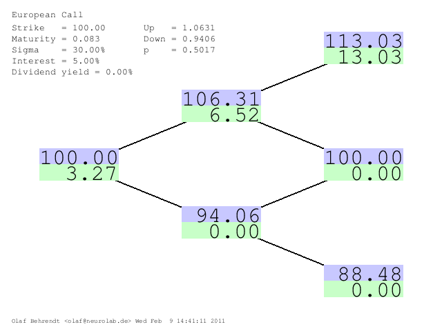
Apart from rounding effects the above calculation can be followed on the graphic created by the online calculator below (prices scaled by 100).

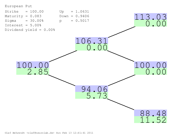
It is easy to calculate bigger trees. We start on the right hand side and calculate the values for the second last nodes using the rightmost single-step trees the same way we did before. Then we proceed one step further to the left till we end up at the root node. Here is an example using the identical parameters above but using a two time-steps tree.

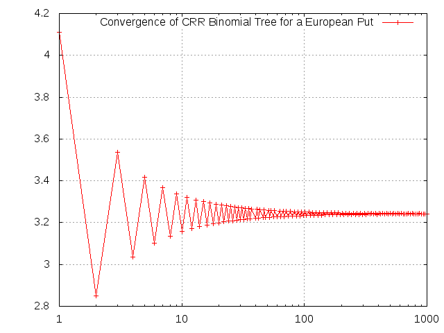
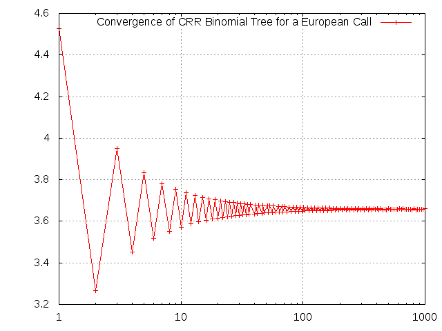
Another interesting issue is the convergence to the theoretical true value which is the Black-Scholes-Price (using the DerivaGem v1.53 accompanying John Hull's book, the exact analytic value is 3.6584956 the binomial tree simulator gives 3.660396 for a 1000 time-steps tree).

European Put

An European put option gives the holder the right to sell the underlying asset at a certain price at a certain time. Its payoff-function is given by $\max(K-S_T,0)$ so that the holder only receives a payoff when the asset price is below the strike price at the maturity of the option.

Now lets assume the following (same as in the above call example) values $$ S_0 = 1,\ K=1,\ T=1/12=0.0833,\ r = 5\%,\ \sigma=30\% $$

Since the valuation is analogous to the above call example (only the payoff-function changed) we only show the output from the online calculator.